Examples¶

These examples show many different ways to use ProxImaL. The Basic examples section shows how to solve some common optimization problems in ProxImaL. The Advanced examples and Real-world applications sections contains more complex examples aimed at experts in convex optimization.

Basic examples¶

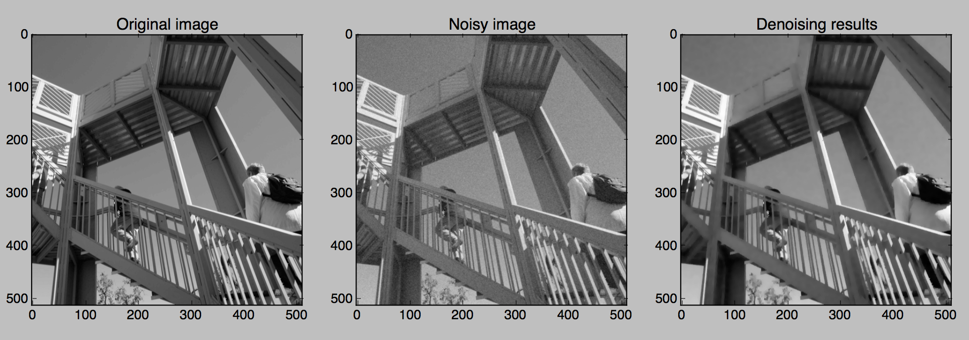
Total variation denoising¶

Signal distortion model:

\[\min_u \| u - b \|_2^2 + 0.1 \| \nabla_x u \|_1 + 0.1 \| \nabla_y u \|_1 + \mathtt{nonneg}(u)\]

Textual representation in ProxImaL:

prob = Problem(
    sum_squares(u - b / 255) + .1 * norm1(grad(u)) + nonneg(u))

Example code: https://github.com/comp-imaging/ProxImaL/blob/master/proximal/examples/basic_denoise.py

Expected output:

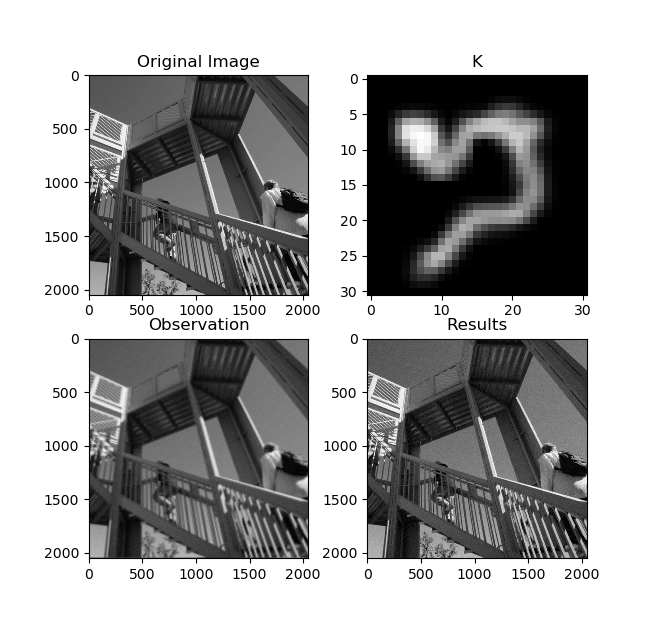
TV-regularized image deconvolution¶

Signal distortion model:

\[\min_u \| \mathtt{conv}(k, u) - b \|_2^2 + \lambda \| \nabla u \|_1\]

Textual representation in ProxImaL:

prob = Problem(
    sum_squares(conv(K, u, dims=2) - b) +
    lambda_tv * group_norm1(grad(u, dims=2), [2]),
)

Example code: https://github.com/comp-imaging/ProxImaL/blob/master/proximal/examples/test_deconv.py

Expected output:

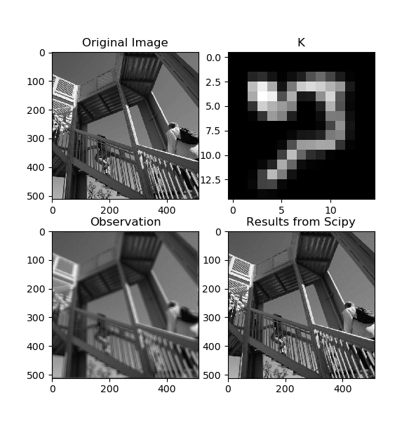
Total variation denoising with multiplicative Poisson noise¶

Signal distortion model:

\[\min_u \| u , b \|_\mathtt{Poisson} + \lambda \| \nabla u \|_1\]

Textual representation in ProxImaL:

prob = Problem([
    poisson_norm(conv(K, u), b),
    lambda_tv * group_norm1(grad(u, dims=2), [2])
])

Example code: https://github.com/comp-imaging/ProxImaL/blob/master/proximal/examples/test_poisson.py

Expected output:

Advanced examples¶

Horn-Schunck optical flow algorithm¶

Signal distortion model:

\[\min_{\{u, v\}} \| \mathtt{Diag}(f_x) u + \mathtt{Diag}(f_y) v - f_t \|_2^2 + \alpha \| \nabla u \|_2^2 + \alpha \| \nabla v \|_2^2.\]

Textual representation in ProxImaL:

prob = px.Problem([
    alpha * px.sum_squares(px.grad(u)),
    alpha * px.sum_squares(px.grad(v)),
    px.sum_squares(px.mul_elemwise(fx, u) + px.mul_elemwise(fy, v) + ft,),
])

Example code: https://github.com/comp-imaging/ProxImaL/blob/master/proximal/examples/test_optical_flow.py

Expected output:

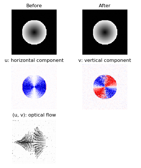
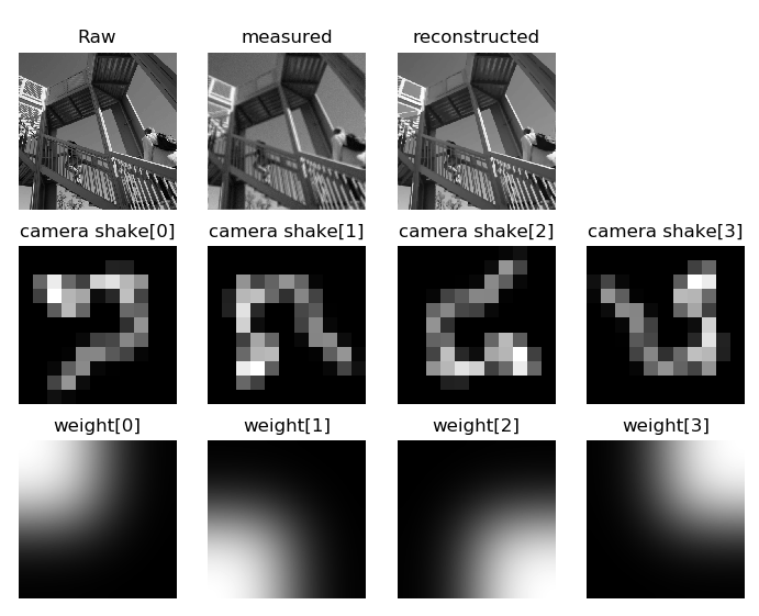
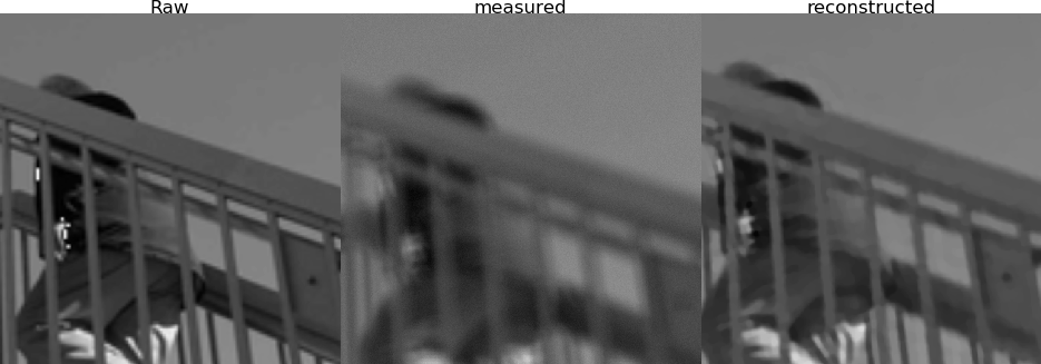
Image deconvolution with spatial varying point spread functions (SV-PSFs)¶

References: Denis, L., Thiébaut, E., Soulez, F. et al. Fast Approximations of Shift-Variant Blur. Int J Comput Vis 115, 253–278 (2015). https://doi.org/10.1007/s11263-015-0817-x

Signal distortion model:

\[\min_u \left\Vert \sum_{i=1}^N \mathtt{conv}[h_i, \mathrm{Diag}(w_i) u] - b \right\Vert_2^2 + \mu \alpha \Vert \nabla u \Vert_1 + \mu (1 - \alpha) \Vert \nabla u \Vert_2^2.\]

Textual representation in ProxImaL:

grad_term = grad(u)

prob = Problem([
    sum_squares(
        sum([
            conv(psf_modes[..., i], mul_elemwise(weights[..., i], u))
            for i in range(n_psf)
        ]) - raw_image
    ),
    lambda_tv * alpha * group_norm1(grad_term, group_dims=[2]),
    lambda_tv * (1.0 - alpha) * sum_squares(grad_term),
])

Example code: https://github.com/comp-imaging/ProxImaL/blob/master/proximal/examples/test_deconv_sv_psf.py

Expected output:

Joint image super-resolution and phase retrieval with Fourier Ptychographic microscopy (FPM)¶

References:

Problem formulation for weak phase objects: Y. Huang, A.C.S. Chan, A. Pan, and C. Yang, “Memory-efficient, Global Phase-retrieval of Fourier Ptychography with Alternating Direction Method,” in Imaging and Applied Optics 2019 (COSI, IS, MATH, pcAOP), OSA Technical Digest (Optica Publishing Group, 2019), paper CTu4C.2. https://doi.org/10.1364/COSI.2019.CTu4C.2
Derivation of the proximal operator of the complex-valued Poisson norm: Hanfei Yan 2020 New J. Phys. 22 023035. https://doi.org/10.1088/1367-2630/ab704e
Imaging instrument specifications and the lens calibration method: A.C.S. Chan, J Kim, A Pan, H Xu, D Nojima, C Hale, S Wang, C Yang, “Parallel Fourier ptychographic microscopy for high-throughput screening with 96 cameras (96 Eyes)” Scientific Reports 9, 11114 (2019). http://dx.doi.org/10.1038/s41598-019-47146-z
Raw data: https://academictorrents.com/details/c95c06e98a74a580ccbcceafdc1188ea144021c8

Signal distortion model:

\[\def\Fourier{\mathbf{F}} \def\Pupil{\mathbf{P}} \def\Shift{\mathbf{S}} \def\Bayer{\mathbf{M}_\mathrm{Bayer,G}} \def\Nonneg{\mathcal{I}_+} \hat u = \arg \min_{u \in \mathbb{C}} \sum_{j=1}^K \left\Vert \Bayer | \Fourier^T \Pupil \Shift_j \Fourier u |^2 , b_j \right\Vert_\mathrm{Poisson} + 0.07 \Vert u - (1 + 0\mathrm{j}) \Vert_2^2 + \Nonneg [ \mathrm{Im}(u) ].\]

Textual representation in ProxImaL:

problem = Problem(
    weighted_poisson_phase_norm(
        bayer_mask_green_channel,
        ptychography(u) * sqrt(1e3),
        simulated_lowres * 1e3,
    ) +
    sum_squares(u - 1.0) * 0.07 +
    nonneg(u),
)

Example code: https://github.com/comp-imaging/ProxImaL/blob/master/proximal/examples/fourier-ptychography.py

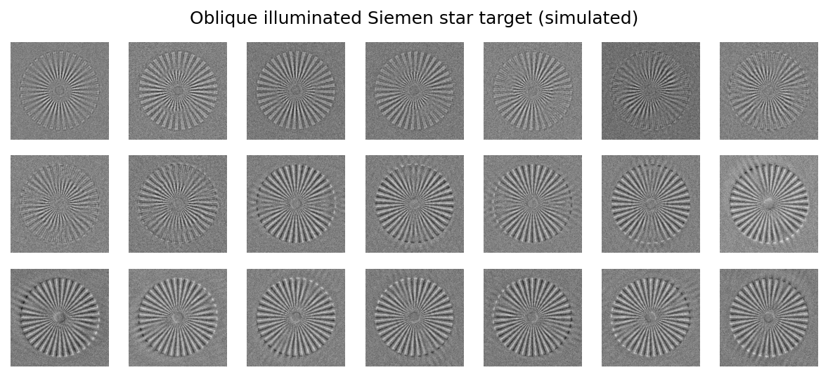
../_images/fpm-inputs.png — Oblique illuminated Siemen star resolution target (simulated):¶

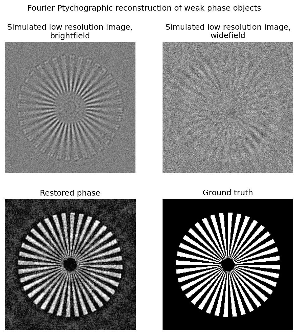
../_images/fpm-outputs.png — Fourier ptychographic phase retrieval results, compared to ground truth.¶

Real-world applications¶

Ptychographical phase retrieval for remote sensing;
Fourier ptychographic microscopy (FPM) for stain-free biological cell culture;
Bayer filter de-interleaving of raw pixels from CMOS image sensors;

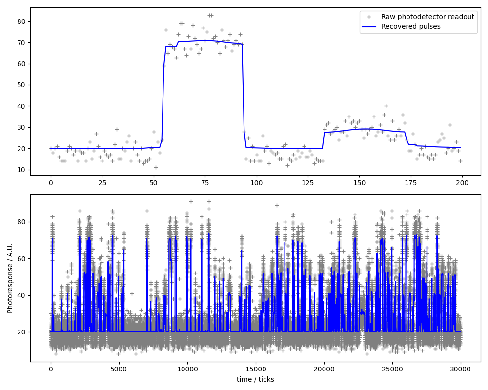
Pulse calling of single-molecule events¶

Reference: Brian D. Reed et al., Real-time dynamic single-molecule protein sequencing on an integrated semiconductor device. Science 378, 186-192(2022). DOI: https://doi.org/10.1126/science.abo7651

Subset of raw data retrieved on July 16, 2023, from https://zenodo.org/records/6789017 .

Warning

The original pulse-recovery method was designed for a streaming processor architecture, likely optimized for reconfigurable hardware having fixed-point arithmetic such as FPGAs. The convex-optimization approach implemented here instead processes data in batches of roughly 30,000 samples and is better suited to GPU execution having single/half-precision floating point arithmetic. Batch-based processing may introduce boundary artifacts, reflecting a trade-off inherent to this non-streaming formulation.

Signal distortion model:

\[\min_u \| u - (b - 20)/128 \|_2^2 + 0.4 \| \nabla u \|_1 + \mathtt{nonneg}(u)\]

Textual representation in ProxImaL:

prob = Problem(
    sum_squares(u - (b - 20.0) / 255.0) + 0.4 * norm1(grad(u)) + nonneg(u))

Example code: https://github.com/comp-imaging/ProxImaL/blob/master/proximal/examples/test_pulse_calling.py

Expected output:

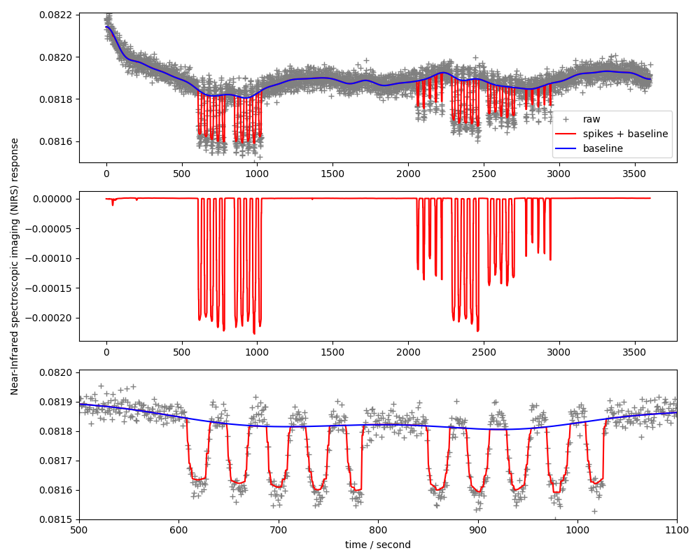
Spike-baseline signal separation of time-lapse signals¶

Reference: I. W. Selesnick, H. L. Graber, D. S. Pfeil and R. L. Barbour, “Simultaneous Low-Pass Filtering and Total Variation Denoising,” in IEEE Transactions on Signal Processing, vol. 62, no. 5, pp. 1109-1124, March1, 2014, https://doi.org/10.1109/TSP.2014.2298836

Signal distortion model:

\[\min_{u,v} \| \mathrm{DCT}^{-1}(v) - u - b \|_2^2 + 0.16 \Vert \nabla u \Vert_1 + 0.04 \Vert u \Vert_1 + \mathtt{nonneg}(u)\]

Textual representation in ProxImaL:

prob = Problem([
        sum_squares(idct_op(baseline) - spikes - measurement),
        0.16 * norm1(grad(spikes)),
        0.04 * norm1(spikes),
        nonneg(u),
])

Example code: https://github.com/comp-imaging/ProxImaL/blob/master/proximal/examples/near-infrared-spectroscopic-imaging.py

Expected output:

Pixel super-resolution of oil emulsion droplets under high-speed camera¶

References: A.C.S. Chan, H.C. Ng, S.C.V. Bogaraju, H.K.H. So, E.Y. Lam, and K.K. Tsia, “All-passive pixel super-resolution of time-stretch imaging,” Scientific Reports, vol. 7, no. 44608, 2017. DOI: http://dx.doi.org/10.1038/srep44608.

Note

The original pixel super-resolution algorithm is meant for a streaming processor architecture, likely optimized for reconfigurable hardware having fixed-point arithmetic such as FPGAs. The convex-optimization approach implemented here instead processes data in batches of roughly 1000 raster scan lines, and is better suited to GPU execution having single/half-precision floating point arithmetic. Batch-based processing may introduce boundary artifacts, reflecting a trade-off inherent to this non-streaming formulation.

Refer to the following article for the baremetal FPGA implementation: Shi R, Wong JSJ, Lam EY, Tsia KK, So HK. A Real-Time Coprime Line Scan Super-Resolution System for Ultra-Fast Microscopy. IEEE Trans Biomed Circuits Syst. 2019 Aug;13(4):781-792. doi: https://doi.org/10.1109/TBCAS.2019.2914946.

Raw data: http://academictorrents.com/details/a8d14f22c9ce1cc59c9f480df5deb0f7e94861f4

Signal distortion model:

\[\min_u \left\Vert \mathbf{M} [\mathbf{W} (u + u_0) - b] \right\Vert_2^2 + 0.005 \| \nabla u \|_{2,1}.\]

Textual representation in ProxImaL:

prob = Problem(
    sum_squares(
        mul_elemwise(
            mask,
            warp(
                pad(u + u_0, b.shape),
                M,
            ) - b,
        )
    ) +
    5e-3 * group_norm1(grad(u), group_dims=[2]),
)

Example code: https://github.com/comp-imaging/ProxImaL/blob/master/proximal/examples/test_pixel_sr.py

Warning

Illumination background extraction for u_0 via the one-dimensional Pixel-SR method (aka the equivalent time sampling method), is omitted here for the sake of demonstration.

Expected output: